
An Intuitive Understanding of Word Embeddings: From Count Vectors to Word2Vec
Table of Contents
Introduction
Before we start, have a look at the below examples.
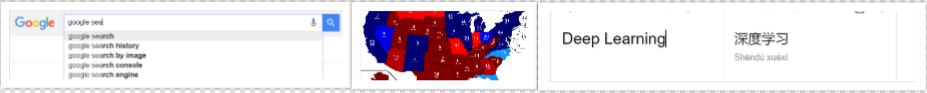
- You open Google and search for a news article on the ongoing Champions trophy and get hundreds of search results in return about it.
- Nate silver analysed millions of tweets and correctly predicted the results of 49 out of 50 states in 2008 U.S Presidential Elections.
- You type a sentence in google translate in English and get an Equivalent Chinese conversion.
So what do the above examples have in common?
You possible guessed it right – TEXT processing. All the above three scenarios deal with humongous amount of text to perform different range of tasks like clustering in the google search example, classification in the second and Machine Translation in the third.
Humans can deal with text format quite intuitively but provided we have millions of documents being generated in a single day, we cannot have humans performing the above the three tasks. It is neither scalable nor effective.

So, how do we make computers of today perform clustering, classification etc on a text data since we know that they are generally inefficient at handling and processing strings or texts for any fruitful outputs?
Sure, a computer can match two strings and tell you whether they are same or not. But how do we make computers tell you about football or Ronaldo when you search for Messi? How do you make a computer understand that “Apple” in “Apple is a tasty fruit” is a fruit that can be eaten and not a company?
The answer to the above questions lie in creating a representation for words that capture their meanings, semantic relationships and the different types of contexts they are used in.
And all of these are implemented by using Word Embeddings or numerical representations of texts so that computers may handle them.
Below, we will see formally what are Word Embeddings and their different types and how we can actually implement them to perform the tasks like returning efficient Google search results.
What are Word Embeddings?
In very simplistic terms, Word Embeddings are the texts converted into numbers and there may be different numerical representations of the same text. But before we dive into the details of Word Embeddings, the following question should be asked – Why do we need Word Embeddings?
As it turns out, many Machine Learning algorithms and almost all Deep Learning Architectures are incapable of processing strings or plain text in their raw form. They require numbers as inputs to perform any sort of job, be it classification, regression etc. in broad terms. And with the huge amount of data that is present in the text format, it is imperative to extract knowledge out of it and build applications. Some real world applications of text applications are – sentiment analysis of reviews by Amazon etc., document or news classification or clustering by Google etc.
Let us now define Word Embeddings formally. A Word Embedding format generally tries to map a word using a dictionary to a vector. Let us break this sentence down into finer details to have a clear view.
Take a look at this example – sentence=“Word Embeddings are Word converted into numbers”
A word in this sentence may be “Embeddings” or “numbers ” etc.
A dictionary may be the list of all unique words in the sentence. So, a dictionary may look like – [‘Word’,’Embeddings’,’are’,’Converted’,’into’,’numbers’]
A vector representation of a word may be a one-hot encoded vector where 1 stands for the position where the word exists and 0 everywhere else. The vector representation of “numbers” in this format according to the above dictionary is [0,0,0,0,0,1] and of converted is[0,0,0,1,0,0].
This is just a very simple method to represent a word in the vector form. Let us look at different types of Word Embeddings or Word Vectors and their advantages and disadvantages over the rest.
Different types of Word Embeddings
The different types of word embeddings can be broadly classified into two categories-
- Frequency based Embedding
- Prediction based Embedding
Let us try to understand each of these methods in detail.
Frequency based Embedding
There are generally three types of vectors that we encounter under this category.
- Count Vector
- TF-IDF Vector
- Co-Occurrence Vector
Let us look into each of these vectorization methods in detail.
Count Vector
Consider a Corpus C of D documents \(\{d_1,d_2,\cdots,d_D\}\) and N unique tokens extracted out of the corpus C. The N tokens will form our dictionary and the size of the Count Vector matrix M will be given by \(D\times N\). Each row in the matrix M contains the frequency of tokens in document D(i).
Let us understand this using a simple example.
D1: He is a lazy boy. She is also lazy.
D2: Neeraj is a lazy person.
The dictionary created may be a list of unique tokens(words) in the corpus =[“He”, “She”, “lazy”, “boy”, “Neeraj”, “person”]
Here, D=2, N=6
The count matrix M of size 2 X 6 will be represented as –
| He | She | lazy | boy | Neeraj | person | |
|---|---|---|---|---|---|---|
| D1 | 1 | 1 | 2 | 1 | 0 | 0 |
| D2 | 0 | 0 | 1 | 0 | 1 | 1 |
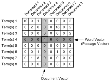
Now, a column can also be understood as word vector for the corresponding word in the matrix M. For example, the word vector for “lazy” in the above matrix is [2,1] and so on.Here, the rows correspond to the documents in the corpus and the columns correspond to the tokens in the dictionary. The second row in the above matrix may be read as – D2 contains “lazy”: once, “Neeraj”: once and “person” once.
Now there may be quite a few variations while preparing the above matrix M. The variations will be generally in-
- The way dictionary is prepared.
Why? Because in real world applications we might have a corpus which contains millions of documents. And with millions of document, we can extract hundreds of millions of unique words. So basically, the matrix that will be prepared like above will be a very sparse one and inefficient for any computation. So an alternative to using every unique word as a dictionary element would be to pick say top 10,000 words based on frequency and then prepare a dictionary. - The way count is taken for each word.
We may either take the frequency (number of times a word has appeared in the document) or the presence(has the word appeared in the document?) to be the entry in the count matrix M. But generally, frequency method is preferred over the latter.
Below is a representational image of the matrix M for easy understanding.
TF-IDF vectorization
This is another method which is based on the frequency method but it is different to the count vectorization in the sense that it takes into account not just the occurrence of a word in a single document but in the entire corpus. So, what is the rationale behind this? Let us try to understand.
Common words like “is”, “the”, “a” etc. tend to appear quite frequently in comparison to the words which are important to a document. For example, a document A on Lionel Messi is going to contain more occurences of the word “Messi” in comparison to other documents. But common words like “the” etc. are also going to be present in higher frequency in almost every document.
Ideally, what we would want is to down weight the common words occurring in almost all documents and give more importance to words that appear in a subset of documents.
TF-IDF works by penalising these common words by assigning them lower weights while giving importance to words like “Messi” in a particular document.
So, how exactly does TF-IDF work?
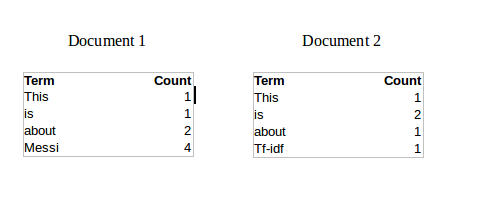
Consider the below sample table which gives the count of terms(tokens/words) in two documents.
Now, let us define a few terms related to TF-IDF.
TF = (Number of times term t appears in a document)/(Number of terms in the document)
So, TF(This,Document1) = 1⁄8
TF(This, Document2)=1⁄5
It denotes the contribution of the word to the document i.e words relevant to the document should be frequent. eg: A document about Messi should contain the word “Messi” in large number.
IDF = log(N/n), where, N is the number of documents and n is the number of documents a term t has appeared in.
So, IDF(This) = log(2⁄2) = 0.
So, how do we explain the reasoning behind IDF? Ideally, if a word has appeared in all the document, then probably that word is not relevant to a particular document. But if it has appeared in a subset of documents then probably the word is of some relevance to the documents it is present in.
Let us compute IDF for the word “Messi”.
IDF(Messi) = log(2⁄1) = 0.301.
Now, let us compare the TF-IDF for a common word “This” and a word “Messi” which seems to be of relevance to Document 1.
TF-IDF(This,Document1) = (1⁄8) * (0) = 0
TF-IDF(This, Document2) = (1⁄5) * (0) = 0
TF-IDF(Messi, Document1) = (4⁄8)*0.301 = 0.15
As, you can see for Document1 , TF-IDF method heavily penalises the word “This” but assigns greater weight to “Messi”. So, this may be understood as “Messi” is an important word for Document1 from the context of the entire corpus.
Co-Occurrence Matrix with a fixed context window
The big idea – Similar words tend to occur together and will have similar context for example – Apple is a fruit. Mango is a fruit.
Apple and mango tend to have a similar context i.e fruit.
Before I dive into the details of how a co-occurrence matrix is constructed, there are two concepts that need to be clarified – Co-Occurrence and Context Window.
Co-occurrence – For a given corpus, the co-occurrence of a pair of words say w1 and w2 is the number of times they have appeared together in a Context Window.
Context Window – Context window is specified by a number and the direction. So what does a context window of 2 (around) means? Let us see an example below,
| Quick | Brown | Fox | Jump | Over | The | Lazy | Dog |
The green words are a 2 (around) context window for the word “Fox” and for calculating the co-occurrence only these words will be counted. Let us see context window for the word “Over”.
| Quick | Brown | Fox | Jump | Over | The | Lazy | Dog |
Now, let us take an example corpus to calculate a co-occurrence matrix.
Corpus = He is not lazy. He is intelligent. He is smart.
| He | is | not | lazy | intelligent | smart | |
| He | 0 | 4 | 2 | 1 | 2 | 1 |
| is | 4 | 0 | 1 | 2 | 2 | 1 |
| not | 2 | 1 | 0 | 1 | 0 | 0 |
| lazy | 1 | 2 | 1 | 0 | 0 | 0 |
| intelligent | 2 | 2 | 0 | 0 | 0 | 0 |
| smart | 1 | 1 | 0 | 0 | 0 | 0 |
Let us understand this co-occurrence matrix by seeing two examples in the table above. Red and the blue box.
Red box- It is the number of times “He” and “is” have appeared in the context window 2 and it can be seen that the count turns out to be 4. The below table will help you visualise the count.
| He | is | not | lazy | He | is | intelligent | He | is | smart |
| He | is | not | lazy | He | is | intelligent | He | is | smart |
| He | is | not | lazy | He | is | intelligent | He | is | smart |
| He | is | not | lazy | He | is | intelligent | He | is | smart |
while the word “lazy” has never appeared with “intelligent” in the context window and therefore has been assigned 0 in the blue box.
Variations of Co-occurrence Matrix
Let’s say there are V unique words in the corpus. So Vocabulary size = V. The columns of the Co-occurrence matrix form the context words. The different variations of Co-Occurrence Matrix are-
- A co-occurrence matrix of size V X V. Now, for even a decent corpus V gets very large and difficult to handle. So generally, this architecture is never preferred in practice.
- A co-occurrence matrix of size V X N where N is a subset of V and can be obtained by removing irrelevant words like stopwords etc. for example. This is still very large and presents computational difficulties.
But, remember this co-occurrence matrix is not the word vector representation that is generally used. Instead, this Co-occurrence matrix is decomposed using techniques like PCA, SVD etc. into factors and combination of these factors forms the word vector representation.
Let me illustrate this more clearly. For example, you perform PCA on the above matrix of size VXV. You will obtain V principal components. You can choose k components out of these V components. So, the new matrix will be of the form \(V\times k\).
And, a single word, instead of being represented in V dimensions will be represented in k dimensions while still capturing almost the same semantic meaning. k is generally of the order of hundreds.
So, what PCA does at the back is decompose Co-Occurrence matrix into three matrices, U,S and V where U and V are both orthogonal matrices. What is of importance is that dot product of U and S gives the word vector representation and V gives the word context representation.

Advantages of Co-occurrence Matrix
- It preserves the semantic relationship between words. i.e man and woman tend to be closer than man and apple.
- It uses SVD at its core, which produces more accurate word vector representations than existing methods.
- It uses factorization which is a well-defined problem and can be efficiently solved.
- It has to be computed once and can be used anytime once computed. In this sense, it is faster in comparison to others.
Disadvantages of Co-Occurrence Matrix
- It requires huge memory to store the co-occurrence matrix. But, this problem can be circumvented by factorizing the matrix out of the system for example in Hadoop clusters etc. and can be saved.
Prediction based Vector
Pre-requisite: This section assumes that you have a working knowledge of how a neural network works and the mechanisms by which weights in an NN are updated. If you are new to Neural Network, I would suggest you go through this awesome article by Sunil to gain a very good understanding of how NN works.
So far, we have seen deterministic methods to determine word vectors. But these methods proved to be limited in their word representations until Mitolov etc. el introduced word2vec to the NLP community. These methods were prediction based in the sense that they provided probabilities to the words and proved to be state of the art for tasks like word analogies and word similarities. They were also able to achieve tasks like King -man +woman = Queen, which was considered a result almost magical. So let us look at the word2vec model used as of today to generate word vectors.
Word2vec is not a single algorithm but a combination of two techniques – CBOW(Continuous bag of words) and Skip-gram model. Both of these are shallow neural networks which map word(s) to the target variable which is also a word(s). Both of these techniques learn weights which act as word vector representations. Let us discuss both these methods separately and gain intuition into their working.
CBOW(Continuous Bag of words)
The way CBOW work is that it tends to predict the probability of a word given a context. A context may be a single word or a group of words. But for simplicity, I will take a single context word and try to predict a single target word.
Suppose, we have a corpus C = “Hey, this is sample corpus using only one context word.” and we have defined a context window of 1. This corpus may be converted into a training set for a CBOW model as follow. The input is shown below. The matrix on the right in the below image contains the one-hot encoded from of the input on the left.
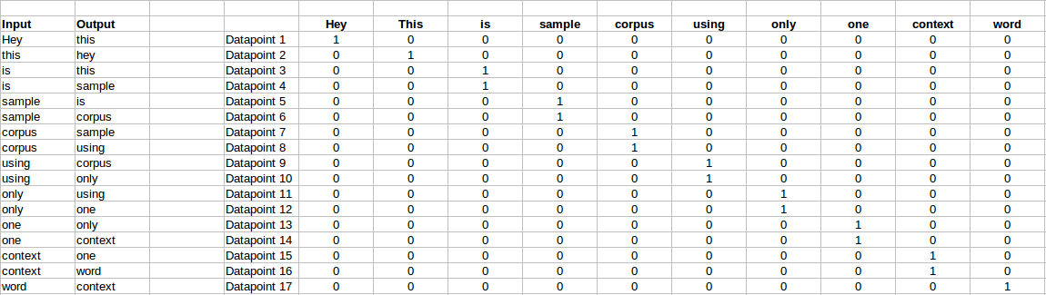
The target for a single datapoint say Datapoint 4 is shown as below
| Hey | this | is | sample | corpus | using | only | one | context | word |
|---|---|---|---|---|---|---|---|---|---|
| 0 | 0 | 0 | 1 | 0 | 0 | 0 | 0 | 0 | 0 |
This matrix shown in the above image is sent into a shallow neural network with three layers: an input layer, a hidden layer and an output layer. The output layer is a softmax layer which is used to sum the probabilities obtained in the output layer to 1. Now let us see how the forward propagation will work to calculate the hidden layer activation.
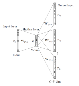
Let us first see a diagrammatic representation of the CBOW model.
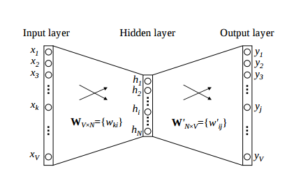
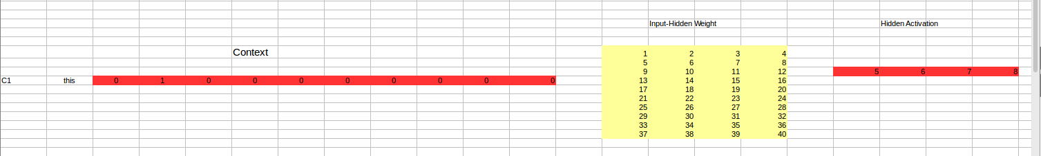
The matrix representation of the above image for a single data point is below.
The flow is as follows:
- The input layer and the target, both are one- hot encoded of size \([1\times V]\). Here V=10 in the above example.
- There are two sets of weights. one is between the input and the hidden layer and second between hidden and output layer.
Input-Hidden layer matrix size =\([V\times N]\), hidden-Output layer matrix size =\([N\times V]\) : Where N is the number of dimensions we choose to represent our word in. It is arbitary and a hyper-parameter for a Neural Network. Also, N is the number of neurons in the hidden layer. Here, N=4. - There is a no activation function between any layers.( More specifically, I am referring to linear activation)
- The input is multiplied by the input-hidden weights and called hidden activation. It is simply the corresponding row in the input-hidden matrix copied.
- The hidden input gets multiplied by hidden- output weights and output is calculated.
- Error between output and target is calculated and propagated back to re-adjust the weights.
- The weight between the hidden layer and the output layer is taken as the word vector representation of the word.
We saw the above steps for a single context word. Now, what about if we have multiple context words? The image below describes the architecture for multiple context words.
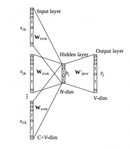
Below is a matrix representation of the above architecture for an easy understanding.
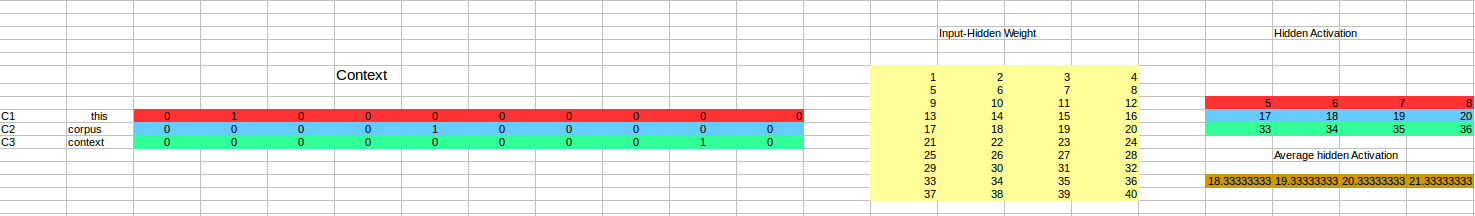
The image above takes 3 context words and predicts the probability of a target word. The input can be assumed as taking three one-hot encoded vectors in the input layer as shown above in red, blue and green.
So, the input layer will have 3\([1\times V]\) Vectors in the input as shown above and 1\([1\times V]\) in the output layer. Rest of the architecture is same as for a 1-context CBOW.
The steps remain the same, only the calculation of hidden activation changes. Instead of just copying the corresponding rows of the input-hidden weight matrix to the hidden layer, an average is taken over all the corresponding rows of the matrix. We can understand this with the above figure. The average vector calculated becomes the hidden activation. So, if we have three context words for a single target word, we will have three initial hidden activations which are then averaged element-wise to obtain the final activation.
In both a single context word and multiple context word, I have shown the images till the calculation of the hidden activations since this is the part where CBOW differs from a simple MLP network. The steps after the calculation of hidden layer are same as that of the MLP as mentioned in this article – Understanding and Coding Neural Networks from scratch.
The differences between MLP and CBOW are mentioned below for clarification:
- The objective function in MLP is a MSE(mean square error) whereas in CBOW it is negative log likelihood of a word given a set of context i.e -log(p(wo/wi)), where p(wo/wi) is given as
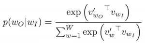
wo : output word
wi: context words
- The gradient of error with respect to hidden-output weights and input-hidden weights are different since MLP has sigmoid activations(generally) but CBOW has linear activations. The method however to calculate the gradient is same as an MLP.
Advantages of CBOW:
- Being probabilistic is nature, it is supposed to perform superior to deterministic methods(generally).
- It is low on memory. It does not need to have huge RAM requirements like that of co-occurrence matrix where it needs to store three huge matrices.
Disadvantages of CBOW:
- CBOW takes the average of the context of a word (as seen above in calculation of hidden activation). For example, Apple can be both a fruit and a company but CBOW takes an average of both the contexts and places it in between a cluster for fruits and companies.
- Training a CBOW from scratch can take forever if not properly optimized.
Skip–Gram model
Skip–gram follows the same topology as of CBOW. It just flips CBOW’s architecture on its head. The aim of skip-gram is to predict the context given a word. Let us take the same corpus that we built our CBOW model on. C=“Hey, this is sample corpus using only one context word.” Let us construct the training data.
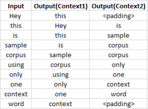
The input vector for skip-gram is going to be similar to a 1-context CBOW model. Also, the calculations up to hidden layer activations are going to be the same. The difference will be in the target variable. Since we have defined a context window of 1 on both the sides, there will be “two” one hot encoded target variables and “two” corresponding outputs as can be seen by the blue section in the image.
Two separate errors are calculated with respect to the two target variables and the two error vectors obtained are added element-wise to obtain a final error vector which is propagated back to update the weights.
The weights between the input and the hidden layer are taken as the word vector representation after training. The loss function or the objective is of the same type as of the CBOW model.
The skip-gram architecture is shown below.
For a better understanding, matrix style structure with calculation has been shown below.
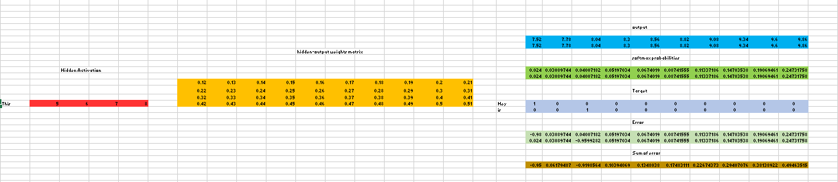
Let us break down the above image.
Input layer size–\([1\times V]\), Input hidden weight matrix size–\([V\times N]\), Number of neurons in hidden layer – N, Hidden-Output weight matrix size–\([N\times V]\), Output layer size–C\([1\times V]\)
In the above example, C is the number of context words=2, V= 10, N=4
- The row in red is the hidden activation corresponding to the input one-hot encoded vector. It is basically the corresponding row of input-hidden matrix copied.
- The yellow matrix is the weight between the hidden layer and the output layer.
- The blue matrix is obtained by the matrix multiplication of hidden activation and the hidden output weights. There will be two rows calculated for two target(context) words.
- Each row of the blue matrix is converted into its softmax probabilities individually as shown in the green box.
- The grey matrix contains the one hot encoded vectors of the two context words(target).
- Error is calculated by substracting the first row of the grey matrix(target) from the first row of the green matrix(output) element-wise. This is repeated for the next row. Therefore, for n target context words, we will have n error vectors.
- Element-wise sum is taken over all the error vectors to obtain a final error vector.
- This error vector is propagated back to update the weights.
Advantages of Skip-Gram Model
- Skip-gram model can capture two semantics for a single word. i.e it will have two vector representations of Apple. One for the company and other for the fruit.
- Skip-gram with negative sub-sampling outperforms every other method generally.
This is an excellent interactive tool to visualise CBOW and skip gram in action. I would suggest you to really go through this link for a better understanding.
Word Embeddings use case scenarios
Since word embeddings or word Vectors are numerical representations of contextual similarities between words, they can be manipulated and made to perform amazing tasks like-
- Finding the degree of similarity between two words.
model.similarity('woman','man')
0.73723527- Finding odd one out.
model.doesnt_match('breakfast cereal dinner lunch';.split())
'cereal'- Amazing things like woman+king-man =queen
model.most_similar(positive=['woman','king'],negative=['man'],topn=1)
queen: 0.508- Probability of a text under the model
model.score(['The fox jumped over the lazy dog'.split()])
0.21
Below is one interesting visualisation of word2vec.
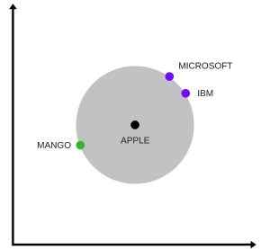
The above image is a t-SNE representation of word vectors in 2 dimension and you can see that two contexts of apple have been captured. One is a fruit and the other company.
- It can be used to perform Machine Translation.
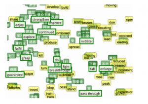
The above graph is a bilingual embedding with chinese in green and english in yellow. If we know the words having similar meanings in chinese and english, the above bilingual embedding can be used to translate one language into the other.
Using pre-trained word vectors
We are going to use google’s pre-trained model. It contains word vectors for a vocabulary of 3 million words trained on around 100 billion words from the google news dataset. The downlaod link for the model is this. Beware it is a 1.5 GB download.
from gensim.models import Word2Vec

#loading the downloaded model
model = Word2Vec.load_word2vec_format('GoogleNews-vectors-negative300.bin', binary=True, norm_only=True)

#the model is loaded. It can be used to perform all of the tasks mentioned above.

# getting word vectors of a word
dog = model['dog']

#performing king queen magic
print(model.most_similar(positive=['woman', 'king'], negative=['man']))

#picking odd one out
print(model.doesnt_match("breakfast cereal dinner lunch".split()))

#printing similarity index
print(model.similarity('woman', 'man'))
Training your own word vectors
We will be training our own word2vec on a custom corpus. For training the model we will be using gensim and the steps are illustrated as below.
word2Vec requires that a format of list of list for training where every document is contained in a list and every list contains list of tokens of that documents. I won’t be covering the pre-preprocessing part here. So let’s take an example list of list to train our word2vec model.
sentence=[["Neeraj","Boy"],["Sarwan","is"],["good","boy"]]
#training word2vec on 3 sentences
model = gensim.models.Word2Vec(sentence, min_count=1,size=300,workers=4)
Let us try to understand the parameters of this model.
sentence – list of list of our corpus
min_count=1 -the threshold value for the words. Word with frequency greater than this only are going to be included into the model.
size=300 – the number of dimensions in which we wish to represent our word. This is the size of the word vector.
workers=4 – used for parallelization
#using the model
#The new trained model can be used similar to the pre-trained ones.
#printing similarity index
print(model.similarity('woman', 'man'))
End Notes
Word Embeddings is an active research area trying to figure out better word representations than the existing ones. But, with time they have grown large in number and more complex. This article was aimed at simplying some of the workings of these embedding models without carrying the mathematical overhead. If you feel think that I was able to clear some of your confusion, comment below. Any changes or suggestions would be welcomed.
Note: We also have a video course on Natural Language Processing covering many NLP topics including word embeddings. Do check it out!